History of atomic models
Ancient Greece (Leucippus and Democritus)
- a thought of the world being composed of small indivisible particles originated at this time
- the theory was not popular and considered heretical later
- atoms were little and invisible for a naked eye and were connected together via small hooks
Early 19th century (John Dalton)
- Dalton ressurected the theory of atoms
- he proposed they were small balls of different colors and sizes
- he based his thinking on many eperiments he did
Later 19th centrury (J. J. Thompson)
- Thompson observed negatively charged particle rays in Crooks tubes, simillair to Helmholtz
- he also later observed positively charged hydrogen atoms in simillair experiments
- he named these tiny particles corpuscules
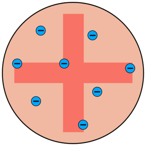
- he proposed a model of atom, where negatively charged particles were equally distributed in a positively charged substance (plum-pudding model)
- the overall charge was neutral and was equally distributed throughout the whole atom
Late 19th century (Ernest Rutherford)
- Rutherford observed that when a this sheet of gold was bombared by alpha particles, they were deflected and their paths were bent
- from this he concluded that he positive part of an atom must be concentrated at one spot in the atom
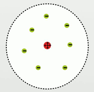
- he proposed an atom with a positively charged nucleus and electrons floating around it
- later his model was refined when isotopes were discovered
Early 20th century (Niels Bohr)
- Bohr refined Rutherford’s model even more by adding distinctive energetic levels at which the electrons orbit
- electrons had energy at these orbits which allowed them to orbit and not simply fall to the positively charged nucleus
- electrons could jump from one energy level to another either emmitting or gaining energy
- the orbits of the atom constituted its electron shell
- this model was later refined even more, adding new ideas, e.g. more than one electron on one orbit, eliprical orbits, etc.
Quantum model of an atom (Erwin Schrödinger)
- Bohr’s model was found to be flawed when new observations were made
- based on calculations made by Schrödinger and his colleagues, a new model was proposed, where electrons are not orbiting atoms in distinct orbits, but rather are spinning and vibrating and some regions around the nucleus
- orbitals - the regions with the highest propability of electron occurence - were proposed
Description of the quantum model of an atom
Quantum numbers
- electrons and their orbitals are described by four quantum numbers
Principal quantum number
- principal quantum number denotes the energy level the electron is on
- it describes the overall energy of an electron
Azimuthal quantum number
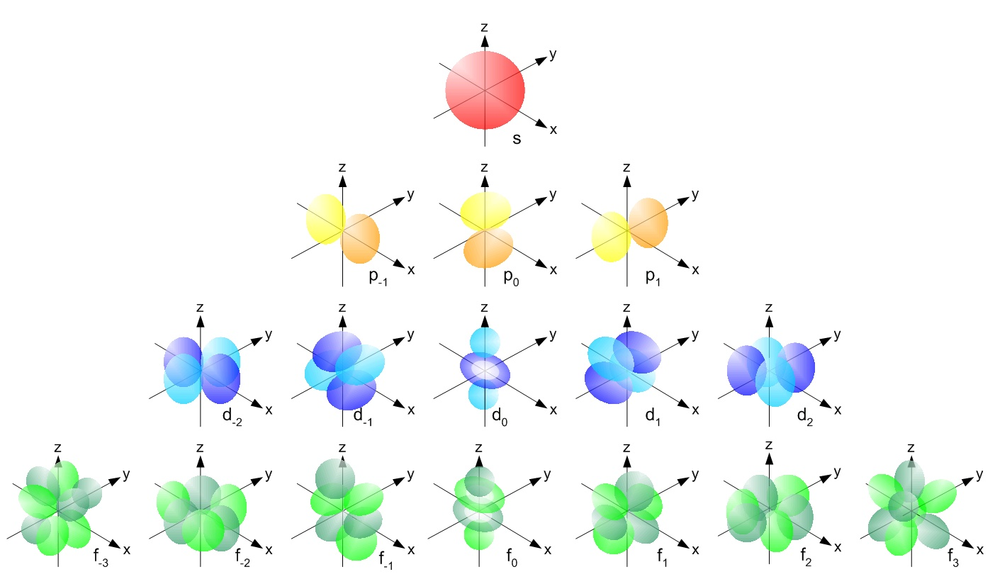
- azimuthal quantum number determines the shape of the orbital the electron is in
- it is written using a letter - s, p, d and f
- each letter corresponds to a different shape
Magnetic quantum number
- magnetic quantum number determines the orientation of the orbital in space
- the number of space orientatons is determined my the shape of the orbital (i.e. the azimuthal quantum number)
- s-orbital has 1 space orientation
- p-orbital has 3 space orientations
- d-orbital has 5 space orientations
- f-orbital has 7 space orientations
Spin quantum number
- spin quantum number determines the spin of an electron
- the spin is either up or down
Electron configuration
- electron configuration is the list of all electrons an atom has in their respective orbitals
Filling orbitals
- how orbitals are filled is determined by three main rules:
Pauli’s exclusion principle
Two electrons cannot occupy the same space; therfore, they must differ at least by their spin quantum number.
Aufbau principle
Electrons first occupy orbitals with the smallest ammount of energy needed.
Hund’s rule
The orbitals with more than one space orientation are filled first with electrons with only one spin in each of the space orientation and then with the other spin.
Writing electron configuration
- electron configuration can be written either symbolically or graphically
- symbolical electron configuration is written as $nl^x$, where $n$ is the principal quantum number, $l$ is the azimuthal quantum number and $x$ is the number of electrons
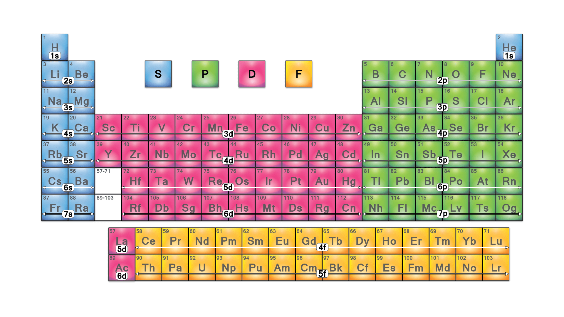
- the main quantum number is the row of the periodic table
- the azimuthal quantum number is the block of the periodic table
Blocks of the periodic table - ex. Electron confuguration of Lithium $$Li:\ 1s^22s^1$$
- the notation can be shorthanded only to valence electrons using the configuration of the previous noble gas
- ex. Shorthanded electron configuration of Sodium $$Na:\ [Ne]3s^1$$
- graphical electron configuration is written as $nl\underline{\uparrow\ }$, where the arrows determine the spin of electrons
- ex. Electron configuration of Oxygen $$O:\ [He]2s\underline{\uparrow\downarrow}\ 2p\underline{\uparrow\downarrow}\ \underline{\uparrow\ }\ \underline{\uparrow\ }$$
Periodic trends
- periodic table of elements is organized in a way that some properties of the elements can be read simply by looking on the table
Highest energy valence orbitals
- periodic table is devided into four blocks
- see here
Atomic mass
- the more nucleons an atom has, the higher its atomic mass
- the further down and to the right we go in the periodic table, the higher the atomic mass
Atomic radius
- the more protons an atom has, the bigger the pull on the electrons around it, hence a smaller atomic radius
- the atomic radius decreases in periods, since the electrons are on one energy level (in the same distance) from the nucleus
- the atomic radius increases in groups, since the outermost electrons are further from the nucleus, because they are on a higher energy level
- the further down and to the left we go in the periodic table, the higher the atomic radius
Ionic radius
- the ionic radius shrinks when electrons are removed and it grows when they are added for the same reasons atomic radius behaves the way it does
- the ionic radius is going to be larger the bigger the difference between the number of electrons and the number of protons gets
First ionization energy
- first ionization energy is the energy needed to remove one (the outermost) electron of an atom
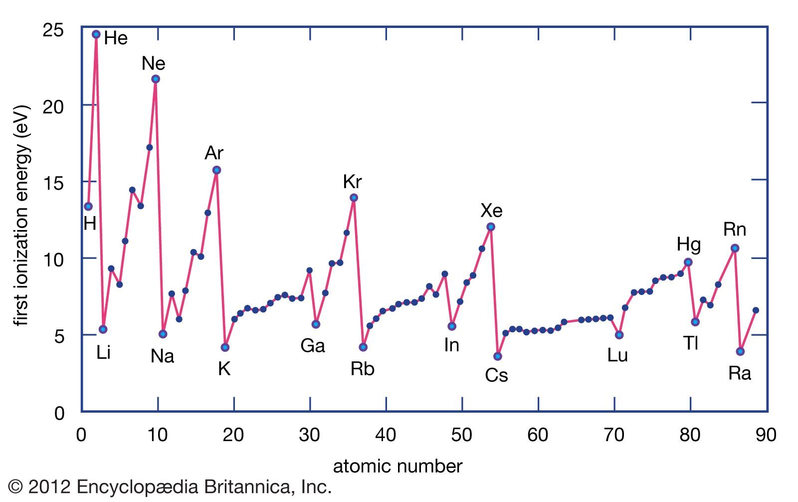
- atoms are most stable when their valence orbitals are either full or half-full
- noble gasses have the highest first ionization energies, because they have their valence orbitals full and thus don’t want to give them up
- alkali metals are only one electron away from reaching a full orbital one energy level lower and thus are glad to give the one electron up
- elements like nitrogen have their valence p-orbital half-full and thus halfway to having a full p-orbital or a full s-orbital, which means they are rather stable and wont give up their electrons as easily as elements like oxygen or fluorine
- the further up and to the right we go in the periodic table, the higher the first ionization energy
Electronegativity $\varkappa$
- electronegativity is the tendency of an atom tu pull electrons of a chemical bond towards itself
- it is related to first ionization energy and electron affinity
- electron affinity is the tendency of an atom to keep its electrons in its electron shell
- electronegativty can be calculated as: $$\varkappa=\cfrac{E_I+E_{EA}}{2}$$
- where:
- $E_I$ is the first ionization energy
- $E_{EA}$ is the electron affinity
- the further up and to the right we go in the periodic table, the higher the electronegativity